Getting Started with Scimap
#!/usr/bin/env python3
# -*- coding: utf-8 -*-
"""
Created on Fri Jun 26 23:11:32 2020
@author: Ajit Johnson Nirmal
Scimap Getting Started tutorial
"""
'\nCreated on Fri Jun 26 23:11:32 2020\n@author: Ajit Johnson Nirmal\nScimap Getting Started tutorial\n'
# Before you start make sure you have installed the following packages
# pip install scimap
# pip install scanpy
# pip install leidenalg
# pip install PyQt5
Tutorial material
You can download the material for this tutorial from the following link:
The presentation files are available here:
Tutorial video
from IPython.display import HTML
HTML('<iframe width="450" height="250" src="https://www.youtube.com/embed/knh5elRksUk" frameborder="0" allow="accelerometer; autoplay; encrypted-media; gyroscope; picture-in-picture" allowfullscreen></iframe>')
# Load necessary libraries
import sys
import os
import anndata as ad
import pandas as pd
import scanpy as sc
import seaborn as sns; sns.set(color_codes=True)

# Import Scimap
import scimap as sm
# Set the working directory
os.chdir ("/Users/aj/Desktop/scimap_tutorial/")
Load data using AnnData
# Load data
data = pd.read_csv ('counts_table.csv') # Counts matrix
meta = pd.read_csv ('meta_data.csv') # Meta data like x and y coordinates

# combine the data and metadata file to generate the AnnData object
adata = ad.AnnData (data)
adata.obs = meta
Print adata to check for it's content
adata
AnnData object with n_obs × n_vars = 4825 × 48
    obs: 'X_centroid', 'Y_centroid', 'Area', 'MajorAxisLength', 'MinorAxisLength', 'Eccentricity', 'Solidity', 'Extent', 'Orientation'
adata.obs # prints the meta data
| X_centroid | Y_centroid | Area | MajorAxisLength | MinorAxisLength | Eccentricity | Solidity | Extent | Orientation | |
|---|---|---|---|---|---|---|---|---|---|
| 0 | 511.555556 | 9.846154 | 117 | 14.532270 | 10.273628 | 0.707261 | 0.959016 | 0.750000 | -0.695369 |
| 1 | 579.330097 | 9.398058 | 103 | 16.056286 | 8.776323 | 0.837396 | 0.903509 | 0.613095 | 1.115707 |
| 2 | 630.958333 | 12.883333 | 120 | 15.222005 | 10.310756 | 0.735653 | 0.975610 | 0.681818 | 0.151616 |
| 3 | 745.194631 | 16.275168 | 149 | 14.380200 | 13.404759 | 0.362027 | 0.967532 | 0.662222 | -0.270451 |
| 4 | 657.173653 | 18.035928 | 167 | 17.675831 | 12.110106 | 0.728428 | 0.943503 | 0.695833 | -0.810890 |
| ... | ... | ... | ... | ... | ... | ... | ... | ... | ... |
| 4820 | 559.597403 | 1091.577922 | 154 | 18.150307 | 11.683288 | 0.765281 | 0.900585 | 0.570370 | -0.342315 |
| 4821 | 619.983871 | 1092.959677 | 248 | 21.734414 | 15.565820 | 0.697912 | 0.864111 | 0.551111 | 1.432242 |
| 4822 | 583.317073 | 1093.573171 | 82 | 12.060039 | 9.539789 | 0.611784 | 0.964706 | 0.630769 | 0.203023 |
| 4823 | 607.064394 | 1101.583333 | 264 | 22.549494 | 15.905321 | 0.708858 | 0.882943 | 0.661654 | 0.691838 |
| 4824 | 641.592486 | 1100.132948 | 346 | 23.149806 | 19.375564 | 0.547257 | 0.945355 | 0.791762 | -1.390516 |
4825 rows × 9 columns
adata.X # prints the counts table
array([[16640.564  ,   719.6325 ,   527.7094 , ...,  1085.735  ,
          218.54701,  3170.47   ],
       [16938.3    ,   686.5534 ,   469.30096, ...,  1075.6407 ,
          164.48544,  3116.767  ],
       [16243.542  ,   819.4167 ,   604.39166, ...,  1164.3917 ,
          227.74167,  3156.1084 ],
       ...,
       [28656.256  ,   878.2561 ,   585.3293 , ...,  1233.183  ,
         1243.5488 ,  3194.195  ],
       [22054.818  ,   685.8485 ,   424.85226, ...,  1031.2424 ,
          313.32574,  3038.8105 ],
       [23992.854  ,   850.25146,   529.89886, ...,  1000.5578 ,
          285.98267,  3087.3005 ]], dtype=float32)
adata.var[0:5] # prints the first 5 channel or marker names
| DNA1 |
|---|
| BG1 |
| BG2 |
| BG3 |
| DNA2 |
You would have noticed that - the data is not in log scale - All the DNA channels are there - The background channels are there If we diretly perform clustering or any other type of analysis, the above mentioned factors may affect the results and so it is recommended to remove them.
Load data using scimap's helper function
Use this if the single-cell data was generated using mcmicro pipeline. With this function though many of the above limitations can be imediately addressed. By default it removes DNA channels and you can pass any channel name into drop_markers parameter inorder to not import them.
image_path = ['/Users/aj/Desktop/scimap_tutorial/mcmicro_output.csv']
adata = sm.pp.mcmicro_to_scimap (image_path, drop_markers = ["PERK", "NOS2","BG1","BG2","BG3","ACTIN"])
Loading mcmicro_output.csv
Check adata contents now as we did previously
adata
AnnData object with n_obs × n_vars = 4825 × 30
    obs: 'X_centroid', 'Y_centroid', 'Area', 'MajorAxisLength', 'MinorAxisLength', 'Eccentricity', 'Solidity', 'Extent', 'Orientation', 'imageid'
    uns: 'all_markers'
adata.X # Will now contain log normalized data
array([[6.3674684, 6.4287267, 7.3826084, ..., 6.990933 , 5.3915663,
        8.061951 ],
       [6.340171 , 6.094227 , 7.339796 , ..., 6.981601 , 5.1088834,
        8.044872 ],
       [6.503502 , 6.3549495, 7.4734573, ..., 7.0608125, 5.4325933,
        8.057412 ],
       ...,
       [6.5583014, 6.660794 , 7.4199724, ..., 7.1181645, 7.1265283,
        8.069404 ],
       [6.3370404, 6.281594 , 7.2397914, ..., 6.939489 , 5.7504296,
        8.01955  ],
       [6.3805585, 6.180567 , 7.2547846, ..., 6.909312 , 5.659422 ,
        8.035377 ]], dtype=float32)
adata.raw.X # contains the raw data
array([[ 581.5812 ,  618.38464, 1606.7778 , ..., 1085.735  ,  218.54701,
        3170.47   ],
       [ 565.8932 ,  442.29126, 1539.3981 , ..., 1075.6407 ,  164.48544,
        3116.767  ],
       [ 666.475  ,  574.3333 , 1759.6833 , ..., 1164.3917 ,  227.74167,
        3156.1084 ],
       ...,
       [ 704.0732 ,  780.1707 , 1667.9878 , ..., 1233.183  , 1243.5488 ,
        3194.195  ],
       [ 564.1212 ,  533.64014, 1392.803  , ..., 1031.2424 ,  313.32574,
        3038.8105 ],
       [ 589.2572 ,  482.2659 , 1413.8584 , ..., 1000.5578 ,  285.98267,
        3087.3005 ]], dtype=float32)
adata.obs # prints the meta data
| X_centroid | Y_centroid | Area | MajorAxisLength | MinorAxisLength | Eccentricity | Solidity | Extent | Orientation | imageid | |
|---|---|---|---|---|---|---|---|---|---|---|
| mcmicro_output_1 | 511.555556 | 9.846154 | 117 | 14.532270 | 10.273628 | 0.707261 | 0.959016 | 0.750000 | -0.695369 | mcmicro_output |
| mcmicro_output_2 | 579.330097 | 9.398058 | 103 | 16.056286 | 8.776323 | 0.837396 | 0.903509 | 0.613095 | 1.115707 | mcmicro_output |
| mcmicro_output_3 | 630.958333 | 12.883333 | 120 | 15.222005 | 10.310756 | 0.735653 | 0.975610 | 0.681818 | 0.151616 | mcmicro_output |
| mcmicro_output_4 | 745.194631 | 16.275168 | 149 | 14.380200 | 13.404759 | 0.362027 | 0.967532 | 0.662222 | -0.270451 | mcmicro_output |
| mcmicro_output_5 | 657.173653 | 18.035928 | 167 | 17.675831 | 12.110106 | 0.728428 | 0.943503 | 0.695833 | -0.810890 | mcmicro_output |
| ... | ... | ... | ... | ... | ... | ... | ... | ... | ... | ... |
| mcmicro_output_4821 | 559.597403 | 1091.577922 | 154 | 18.150307 | 11.683288 | 0.765281 | 0.900585 | 0.570370 | -0.342315 | mcmicro_output |
| mcmicro_output_4822 | 619.983871 | 1092.959677 | 248 | 21.734414 | 15.565820 | 0.697912 | 0.864111 | 0.551111 | 1.432242 | mcmicro_output |
| mcmicro_output_4823 | 583.317073 | 1093.573171 | 82 | 12.060039 | 9.539789 | 0.611784 | 0.964706 | 0.630769 | 0.203023 | mcmicro_output |
| mcmicro_output_4824 | 607.064394 | 1101.583333 | 264 | 22.549494 | 15.905321 | 0.708858 | 0.882943 | 0.661654 | 0.691838 | mcmicro_output |
| mcmicro_output_4825 | 641.592486 | 1100.132948 | 346 | 23.149806 | 19.375564 | 0.547257 | 0.945355 | 0.791762 | -1.390516 | mcmicro_output |
4825 rows × 10 columns
We can use scanpy package to explore the data
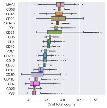
sc.pl.highest_expr_genes(adata, n_top=20, ) # Most expressing proteins
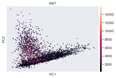
sc.tl.pca(adata, svd_solver='arpack') # peform PCA
sc.pl.pca(adata, color='KI67') # scatter plot in the PCA coordinates
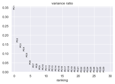
sc.pl.pca_variance_ratio(adata) # PCs to the total variance in the data
# Save the results
adata.write('tutorial_data.h5ad')
This concludes the getting started tutorial, continue with the phenotyping tutorial.